Lesson 07 — Exponential Functions and Their Features
Learners contrast exponential change with linear change — steady multiply versus steady add — and read the features of y = a·bˣ: the initial value a, the growth factor b, the growth rate r = b − 1, and the horizontal asymptote. They model a salary or savings scenario and explain the effect of the base.
Objectives
Objectives
- D05.S2.10.02 Model exponential growth and decay in population, finance, or environmental systems and explain the effect of the rate.
Essential question
What makes exponential change different from steady change, and what do the base, the rate, and the starting value tell me about the future?
Key vocabulary
Materials
Standard materials
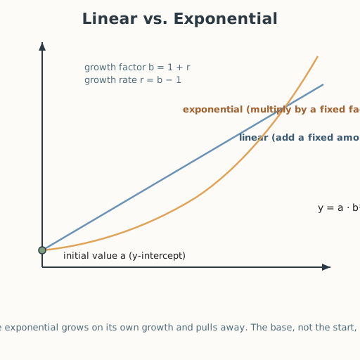
- Linear-vs-exponential chart · 1 per learner Side-by-side tables and graphs of a linear function (steady add) and an exponential function (steady multiply), with features labeled
- Graph paper · 1 per learner
- Math journal · 1 per learner
Low-tech / no-cost
- Two piles of counters Grow one pile by adding a fixed number, the other by doubling — see the difference by hand
- Voice and fingers Chant a linear sequence (add 3) and an exponential one (double) to hear steady add vs. steady multiply
Enriched / lab & device
- Spreadsheet or graphing calculator · 1 per learner or pair To compute many steps of each model and watch the exponential overtake the linear
Works in different contexts
- large-group Build the comparison table whole-class, then learners graph both and pair-share one surprise
- multi-age Younger learners extend a doubling table by hand; older learners derive the formula, find the y-intercept and asymptote, and compare rates
- self-directed A learner follows the worked example, then models a new scenario and checks the features against the chart
- level-grouped Group by fluency with the growth factor from Lesson 3; a ready group extends to finding the doubling time from the rate
- outdoor-only Compare a steady pace (adding equal steps) with a doubling pace outdoors and graph the two distances walked
Lesson 7 — Exponential Functions and Their Features
Summary
Learners contrast exponential change with linear change — steady multiply versus steady add — and read the features of y = a·bˣ: the initial value a, the growth factor b, the growth rate r = b − 1, and the horizontal asymptote. They model a salary or savings scenario and explain the effect of the base.
Objectives
- Model exponential growth and decay and explain the effect of the rate — reading the features of the exponential function. (D05.S2.10.02)
Connection
Two jobs are offered. One pays a steady raise of 1,000 a year; the other pays a 5% raise each year. At first the steady raise looks better. But the 5% job grows on top of its own growth — each year’s raise is bigger than the last — and before long it passes the flat one and keeps climbing. That is the difference between linear change (add a fixed amount) and exponential change (multiply by a fixed factor). Savings, populations, and many natural processes are exponential; reading the base and the rate tells you which curve you are on and where it is headed.
Materials
- Linear-vs-exponential chart
- Graph paper
- Math journal
Preparation
- Copy or draw the linear-vs-exponential chart.
- Retrieval: from Lesson 3, the growth factor b = 1 + r; from Grade 9, linear and exponential functions in context (D05.S2.09.01). Today we formalize the exponential function and its features.
- Prepare the two-offers worked example.
Facilitator note
This lesson is written to the learner (“you”). The idea to land: the exponential function y = a·bˣ grows by a fixed factor each step — its features are the initial value a (the y-intercept), the base b (the growth or decay factor), the rate r = b − 1, and a horizontal asymptote — and the base, not the starting value, decides how fast it runs. Teach with worked examples and guided practice (S-011), and let the linear-vs-exponential contrast do the motivating.
The intellectual lens: “multiply by a fixed factor” is the whole story; every feature is a restatement of it. The critical-thinking lens: ask learners to test which offer is better at year 1, 5, and 20 — a small difference in rate becomes a huge difference over time, so the time horizon matters. The environment lens: exponential growth is the shape behind compounding problems — a warning, not just a number — and it is why small rates over long times deserve respect. The egalitarian lens: two people offered 4% and 6% returns live different futures; who gets which rate is often about access, not merit — a fairness question, not only a math one. Preview: Lesson 8 applies this function to population, finance, and the environment, and to the limit of growth.
Procedure
- Recall (5 min). From Lesson 3, what is the growth factor for a 5% increase? For a 10% decrease? Name the difference between “add 3 each time” and “multiply by 3 each time.”
- Contrast the two shapes (10 min). A linear function adds a fixed amount each step; an exponential function multiplies by a fixed factor each step. On the chart, compare tables: linear (100, 110, 120, …) vs exponential (100, 105, 110.25, …). At first they are close; the exponential curve then bends upward and pulls away.
- Read the features (15 min). Worked example: y = 100 · (1.05)ˣ.
- Initial value a = 100: the y-intercept, the value at x = 0.
- Growth factor b = 1.05: multiply by this each step.
- Growth rate r = b − 1 = 0.05, or 5% per step.
- Asymptote: for decay (0 < b < 1), the curve levels toward y = 0; for growth (b > 1) it climbs without bound.
- Model the two offers (15 min). Offer A: start 100 and add 10 a year (linear). Offer B: start 100 and grow 10% a year (exponential). Build a table for years 0–6, and graph both. Find the year Offer B passes Offer A. State what the base (1.10) and the rate (10%) each mean in words.
- Guided practice (5 min). With a partner, write the exponential function for a quantity that starts at 200 and decays by 20% each step, and state its asymptote.
- Close (5 min). Say in one sentence how the base and the starting value each shape an exponential function’s future.
Differentiation
- Support: Build only the table first and describe the trend in words before graphing.
- Extension: Find the doubling time by trial or reasoning (for b = 1.10, how many steps until roughly 200?), and explain why the base sets it.
Assessment
- Formative (peer + self): Can the learner write an exponential function from a scenario, identify a, b, and r, and explain the effect of changing the rate?
- Portfolio artifact (unit): The linear-vs-exponential chart with the two-offers model, added to the functions toolkit.
Home connection
Ask an adult: if you could have a flat raise or a percentage raise each year, which would you choose and why? Use the two-curves picture to explain what the percentage raise does over many years.
Resources
- On worked examples and guided practice: Kirschner, Sweller & Clark (2006), https://doi.org/10.1207/s15326985ep4102_1 (S-011).